Does BERT Need Clean Data? Part 2 - Classification.

Now for the fun stuff. Light cleaning, heavy cleaning, or no language models at all?

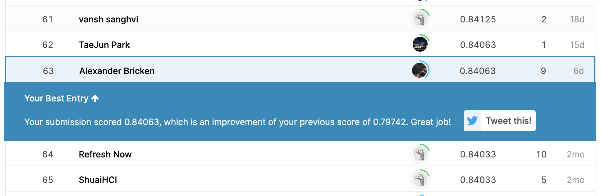
By the end of this article, you should be able to get a top 50 score (84% accuracy) on the NLP Disaster Tweets Kaggle Competition!

Remember, we are trying to classify whether a Tweet designates a disaster (such as a hurricane or forest fire) or doesn’t. The difficulty of this task is a result of the contextual meaning of certain words being different (for example, describing shoes as “fire”).

As mentioned in Part 1, once completing standard text cleaning, we need to decide what machine learning models we want to use and how the input data should look. The goal for this article is to provide a comparison of meta-feature learning using a Deep Neural Network, less intense (lighter) text pre-processing before BERT, and more intense (heavier) text pre-processing before BERT.

As well as this, I will provide an overview of BERT, how it works, and why it is one of the leading language models right now.

Before getting started, we just need to read the pickles from part 1!

# download the pickles saved from part 1
train_df = pd.read_pickle("../data/pickles/clean_train_data.pkl")
test_df = pd.read_pickle("../data/pickles/clean_test_data.pkl")

Now, let’s start with the first way to predict disasters: using meta-features and a neural network.

Meta-Feature Learning

Here, we use just meta-feature data to predict disaster Tweets. This is an alternative method that is being tested. My hypothesis is that it won’t be as good as one of the BERT models, however, it is still interesting to see how it performs. Also, perhaps to improve on BERT in the future, this type of data could be included, so we should test how well our meta-features help distinguish disaster from non-disaster Tweets.

Normalisation

In order to incorporate our meta-features into our modelling, we need to normalise our columns. Normalisation is used to change the integer columns in the dataset to use a common scale, without distorting differences in the ranges of values or losing information. We normalise by using MinMaxScaler(), which allows us to keep the data in the range of [0,1].

# normalise columns
scaler = MinMaxScaler()
final_train_df = scaler.fit_transform(final_train_df)
final_test_df = scaler.fit_transform(final_test_df)

Train-Test Splitting

Before running our Deep Neural Network, we need a way of separating the data so that we can evaluate the model on a test dataset that has not been seen in the train data before. We use sci-kit learn’s train_test_split() function for this.

# train test split
X_train, X_test, y_train, y_test = train_test_split(final_train_df, train_labels, test_size=0.3, random_state=42)

And now that we have a train dataset, a labelled test dataset, and the unlabelled submission test dataset, we can generate our model, fit it on the training data, and test the outcome on our test data, and then run the final model on the submission data before uploading the submissions to Kaggle.

Generating Classification Probabilities Using A Deep Neural Network

I generate a Deep Neural Network by using the Sequential function, allowing me to build the DNN layer-by-layer. The “deep” here means that the NN is connected deeply, as with dense layers the layers receive input from all neurons of the prior layer. I add 5 layers with varying density, using 3 ReLu activation functions (Rectified Linear Activation - this activation function works well in neural networks) and the final sigmoid function that allows me to output the associated probability of an input row being a disaster or non-disaster.

# create DNN
model = Sequential()
model.add(Dense(90, input_dim=9, activation='relu'))
model.add(Dense(120, activation='relu'))
model.add(Dense(100))
model.add(Dense(20, activation='relu'))

model.add(Dense(1, activation='sigmoid'))

# adam optimizer
optimizer = tf.keras.optimizers.Adam(lr=1e-4)

# compile and summarise
model.compile(loss='binary_crossentropy', optimizer=optimizer, metrics=['accuracy'])
model.summary()

# first fit is history1
history = model.fit(X_train, y_train, epochs=100, batch_size=35, validation_data=(X_test, y_test), verbose=1)

Before moving on to the model evaluation, which has the same method across models, the other models’ construction can be shown. Then, a comparison can be made across models in the model evaluation portion.

Light & Heavy Data Cleaning

Some text cleaning might be necessary to optimise BERT performance, but the amount of removal of features of our Tweets is debatable. Because BERT is a model that uses the context of words provided their placement in a sentence in relation to all other words, generally the preservation of such information would be advised. However, in some cases BERT might outperform if data is pruned to a higher degree. In this section light and heavy text cleaning is done. We can then test the performance of either approach in the model evaluation section.

Regex Text Cleaning

Below is some text cleaning. The code is separated into heavy and light portions. In the heavy cleaning, all substitutions are made. In light cleaning, only the light are made (edit the function as you see necessary).

# function taken and modified 
# from https://towardsdatascience.com/cleaning-text-data-with-python-b69b47b97b76

stopwords = set(STOPWORDS)
stopwords.update(["nan"])

def text_clean(x):

    ### Light
    x = x.lower() # lowercase everything
    x = x.encode('ascii', 'ignore').decode()  # remove unicode characters
    x = re.sub(r'https*\S+', ' ', x) # remove links
    x = re.sub(r'http*\S+', ' ', x)
    # cleaning up text
    x = re.sub(r'\'\w+', '', x) 
    x = re.sub(r'\w*\d+\w*', '', x)
    x = re.sub(r'\s{2,}', ' ', x)
    x = re.sub(r'\s[^\w\s]\s', '', x)
    
    ### Heavy
    x = ' '.join([word for word in x.split(' ') if word not in stopwords])
    x = re.sub(r'@\S', '', x)
    x = re.sub(r'#\S+', ' ', x)
    x = re.sub('[%s]' % re.escape(string.punctuation), ' ', x)
    # remove single letters and numbers surrounded by space
    x = re.sub(r'\s[a-z]\s|\s[0-9]\s', ' ', x)

    return x

We apply this function in the following way:

train_df['cleaned_text'] = train_df.text.apply(text_clean)
test_df['cleaned_text'] = test_df.text.apply(text_clean)

Lemmatisation (For Heavy Cleaning)

Just for heavy cleaning, we add one more step: lemmatisation. This is where a library of words is used to remove the inflectional endings of words to return them to their base form, which is known as the lemma. For example, instead of “running” or “runs”, we would just get “run”.

This can sometimes help a model interpret sentences better, so we test it here.

train_list = []
for word in train_text:
    tokens = word_tokenize(word)
    lemmatizer = WordNetLemmatizer()
    lemmatized = [lemmatizer.lemmatize(word) for word in tokens]
    train_list.append(' '.join(lemmatized))

test_list = []
for word in test_text:
    tokens = word_tokenize(word)
    lemmatizer = WordNetLemmatizer()
    lemmatized = [lemmatizer.lemmatize(word) for word in tokens]
    test_list.append(' '.join(lemmatized))

Tokenisation and Embedding

For both light and heavy cleaning, we finally need to tokenise our text data and create appropriate embeddings as a way of including the text data into the machine learning model.

Tokenisation separates a piece of text into tokens. These tokens are words. Embedding a tokenised sentence allows the text data to be turned into numbers that the machine learning model can read. We use the HuggingFace Transformers library to do this.

# we use a pre-trained bert model to tokenise the text
PRE_TRAINED_MODEL_NAME = 'bert-base-uncased'
tokenizer = BertTokenizer.from_pretrained(PRE_TRAINED_MODEL_NAME)

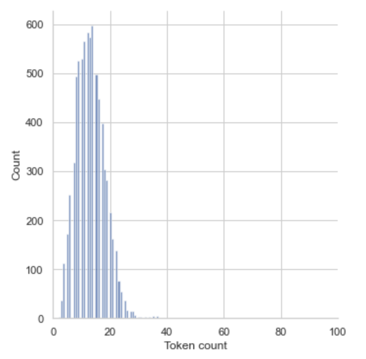
Because BERT works with fixed-length sequences, we need to choose the maximum length of the sequences to best represent the model. By storing the length of each Tweet, we can do this and evaluate the coverage.

token_lens = []
for txt in list(train_list):
    tokens = tokenizer.encode(txt, max_length=512, truncation=True)
    token_lens.append(len(tokens))

sns.displot(token_lens)
plt.xlim([0, 100])
plt.xlabel('Token count')
plt.show()

But what actually is this embedding that BertTokenizer is doing?

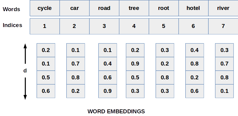
With normal word embedding, we assign some numerical values to each word. An embedding is a d-dimensional vector for each index assigned. See here for more information.

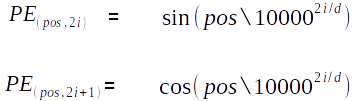
The novelty of a transformer, which is what BERT is built ontop of, is the use of sinusoidal positional encoding for positional indices to word embeddings. By using Sin and Cosine waves for even and odd indices in a tokenised sentence, the same word can have a similar embedding across different lengths of sentences. This provides our embedding no notion of word order and removes duplicate embedding values.

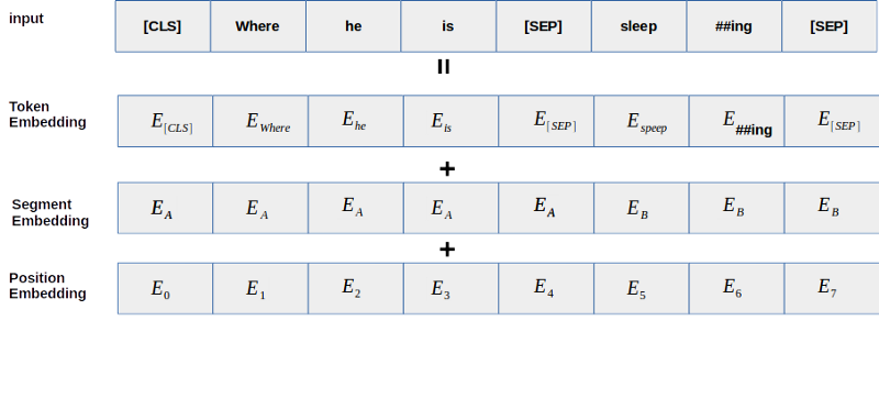
For BERT embeddings, the idea is slightly different to just a transformer. Instead, the model learns the positional embeddings during the training phase and leverages the word-piece tokeniser, where some words are broken into subwords. Thus, rather than just labelling out-of-vocabulary (OOV) words to catch-all tokens, words that are unknown are decomposed into subword and character tokens that the model generates embeddings for. This retains some of the contextual meaning of the original word.

def bert_tokenizer(text):
    encoding = tokenizer.encode_plus(
    text,
    max_length=40,
    truncation=True,
    add_special_tokens=True, # Add '[CLS]' and '[SEP]'
    return_token_type_ids=False,
    pad_to_max_length=True,
    padding='max_length',
    return_attention_mask=True,
    return_tensors='pt',  # Return PyTorch tensors
    )

    return encoding['input_ids'][0], encoding['attention_mask'][0]

We use this function on the train and test datasets:

# train data tokenization
train_tokenized_list = []
train_attn_mask_list = []
for text in list(train_list):
    tokenized_text, attn_mask = bert_tokenizer(text)
    train_tokenized_list.append(tokenized_text.numpy())
    train_attn_mask_list.append(attn_mask.numpy())

# test data tokenization
test_tokenized_list = []
test_attn_mask_list = []
for text in list(test_list):
    tokenized_text, attn_mask = bert_tokenizer(text)
    test_tokenized_list.append(tokenized_text.numpy())
    test_attn_mask_list.append(attn_mask.numpy())

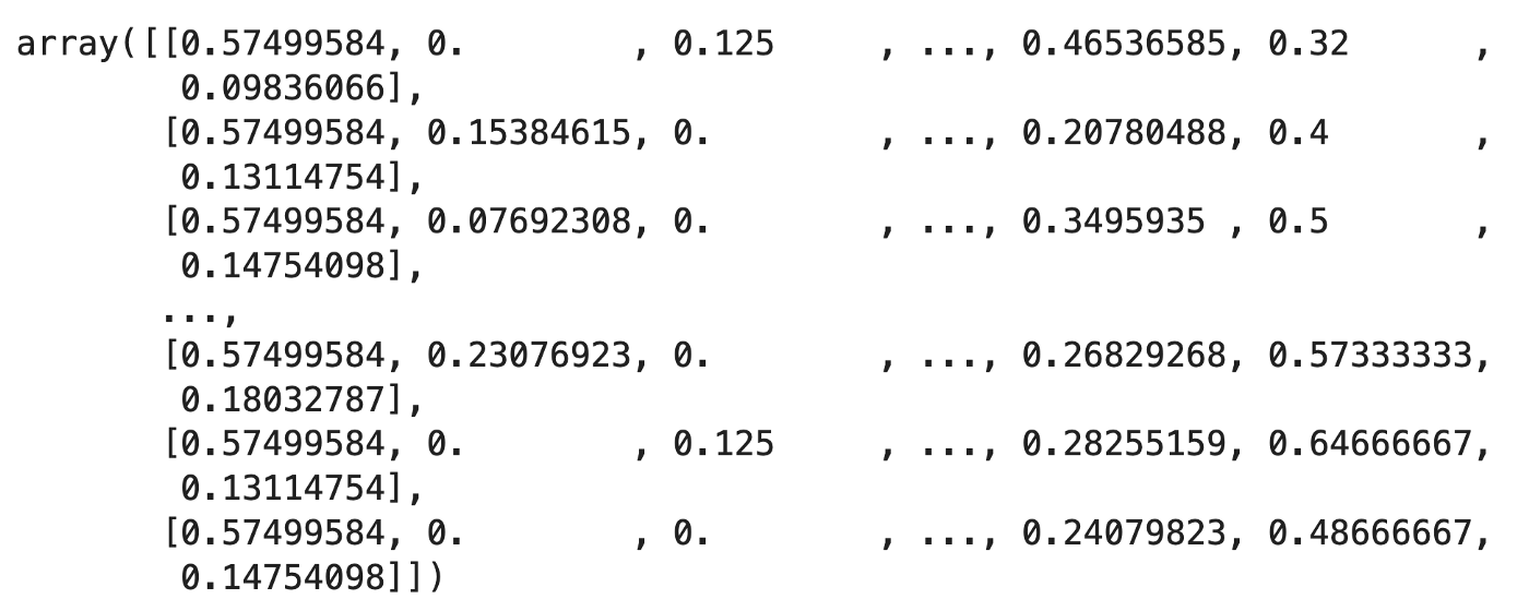
and then can save them as DataFrames to visualise where we are at right now.

train_tokenised_text_df = pd.DataFrame(train_tokenized_list)
test_tokenised_text_df = pd.DataFrame(test_tokenized_list)

Finally, we do another train-test split of our cleaned data (whether it be the heavily cleaned data or the lightly cleaned data).

# train test split
X_train, X_test, y_train, y_test, train_mask, val_mask = train_test_split(train_tokenised_text_df, train_labels, train_attn_mask_list, test_size=0.3, random_state=42)

BERT Modelling

So, what exactly is a BERT model and why have we made all of this fuss about cleaning our data correctly and in different ways?

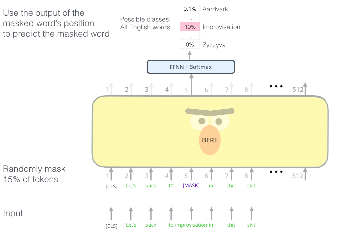
While there are many technical details I could dive into in this paper, I’ll have to refer you to the Google paper. BERT does what the acronym describes: it trains transformers in a bidirectional way. By using a masked language model, which in a simplistic sense is a “leave-one-out” task or Cloze deletion, one word from a sentence is removed, and the model does its best to predict what that word would be. By doing so, and conditioning on both left and right context, a BERT model learns about features of the text and is thus able to distinguish common features of our Tweets beyond just TF-IDF. It uses the context and positioning of words as well.

We use a pretrained BERT model here. It is a good idea to do so because the embeddings of this model have been trained on vast amounts of text data, beyond we could accomplish with this small dataset of Tweets. It is therefore much more efficient and accurate.

num_classes = len(train_labels.unique()) # this is just 2

bert_model = TFBertForSequenceClassification.from_pretrained('bert-base-uncased', num_labels=num_classes)

checkpoint_path = "../models/light_tf_bert.ckpt"
checkpoint_dir = os.path.dirname(checkpoint_path)

model_callback = tf.keras.callbacks.ModelCheckpoint(filepath=checkpoint_path,
                                                 save_weights_only=True,
                                                 verbose=1)

print('\nBert Model', bert_model.summary())

loss = tf.keras.losses.SparseCategoricalCrossentropy(from_logits=True)
metric = tf.keras.metrics.SparseCategoricalAccuracy('accuracy')
optimizer = tf.keras.optimizers.Adam(learning_rate=2e-5,epsilon=1e-08)

bert_model.compile(loss=loss,optimizer=optimizer,metrics=[metric])

Then we fit the model. After testing the model on 10 epochs (which took a long time), it was shown to overfit after the second epoch. Thus, the number of epochs is restricted to 2 as a measure of early stopping. There are various ways to do this, but constraining the number of epochs is the most convenient method for this pre-trained model.

history=bert_model.fit(X_train,
                       y_train,
                       batch_size=32,
                       epochs=2, # in heavy cleaning we use 3 epochs.
                       validation_data=(X_test, y_test),
                       callbacks=[model_callback])

Model Evaluation

To evaluate the models against each other, there are numerous techniques to use. As with any machine learning model, it is best practice to check the accuracy, loss, val accuracy, and val loss. We can do this will the following code:

### Accuracy
plt.figure(figsize=(16, 10))
plt.plot(history.history['accuracy'])
plt.plot(history.history['val_accuracy'])
plt.title('model accuracy')
plt.ylabel('accuracy')
plt.xlabel('epoch')
plt.legend(['train', 'val'], loc='upper left')
plt.show()

### Loss
plt.figure(figsize=(16, 10))
plt.plot(history.history['loss'])
plt.plot(history.history['val_loss'])
plt.title('model loss')
plt.ylabel('loss')
plt.xlabel('epoch')
plt.legend(['train', 'val'], loc='upper left')
plt.show()

Accuracy Graph	Loss Graph

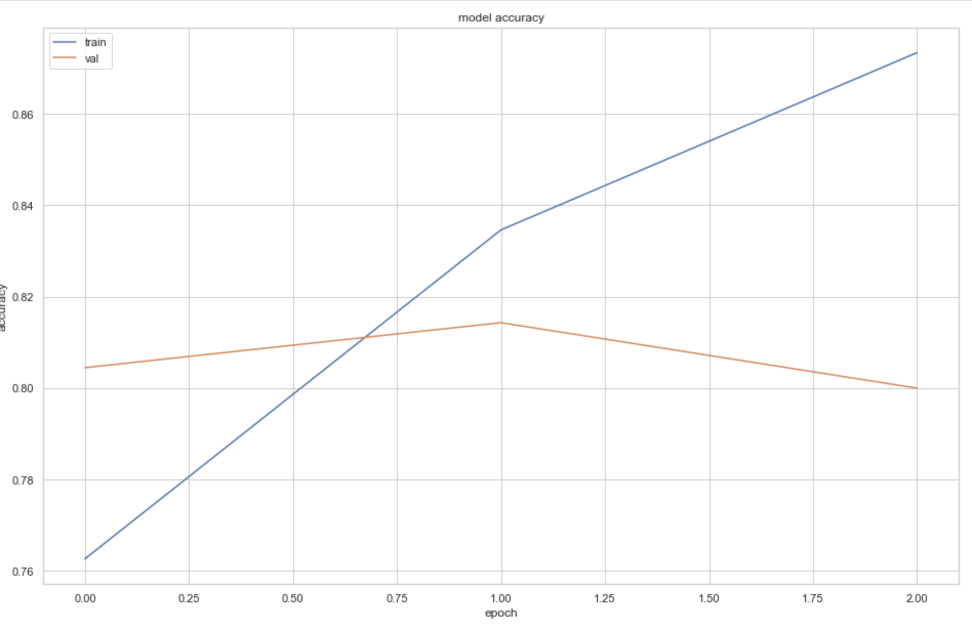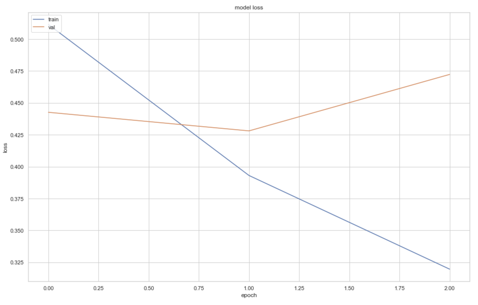These graphs help to understand whether the model is overfitting, underfitting, or a good fit. Given we are using the pre-trained BERT model, we need very few epochs to train the model (see Zhu, J).

After testing my models with both heavy and light cleaning, it is evident that fewer epochs is better for preventing overfitting. This is visualised as the accuracy continues to increase, but val accuracy declines and val loss increases as more epochs are run.

Finally, if we are happy with our models, we can generate our predictions using our test dataset and compare the accuracy to our test dataset labels. By doing so, we find the strongest model and then predict, using that model, on the Kaggle test data and submit to Kaggle.

Predictions

We can predict with any model by running the following code:

# predictions
test_pred = model.predict(X_test)
print(test_pred)

If the output of the prediction is probabilities, we can use this piece of code to convert the output probabilities into 0s and 1s, the binary values of prediction. We split the probabilities at 0.5. Any predictions above 0.5 are labelled as disasters, and below non-disasters.

# this checks if the probability of 
# disaster is above 0.5. If so, we label 1.

test_pred_bool = test_pred.copy().astype(int)
for index in range(len(test_pred)): 
    if test_pred[index]>0.5:
        test_pred_bool[index]=1
    else:
        test_pred_bool[index]=0

final_predictions = test_pred_bool.flatten()

And then for any of our models, we can use a function to evaluate their accuracy by inputting our predictions against the test labels.

# model test function
def eval_model(predictions):
    print(accuracy_score(y_test, predictions))
    # Compute fpr, tpr, thresholds and roc auc
    fpr, tpr, thresholds = roc_curve(np.array(y_test), np.array(predictions))
    roc_auc = auc(fpr, tpr)

    # Plot ROC curve
    plt.plot(fpr, tpr, label='ROC curve (area = %0.3f)' % roc_auc)
    plt.plot([0, 1], [0, 1], 'k--')  # random predictions curve
    plt.xlim([0.0, 1.0])
    plt.ylim([0.0, 1.0])
    plt.xlabel('False Positive Rate or (1 - Specifity)')
    plt.ylabel('True Positive Rate or (Sensitivity)')
    plt.title('Receiver Operating Characteristic')
    plt.legend(loc="lower right")
    plt.show()
    print(classification_report(y_test, np.array(predictions), target_names=["not disaster", "disaster"]))

eval_model(final_predictions)

So, for each of out models we achieve the following results:

DNN Meta-Features	Light Cleaning BERT	Heavy Cleaning BERT

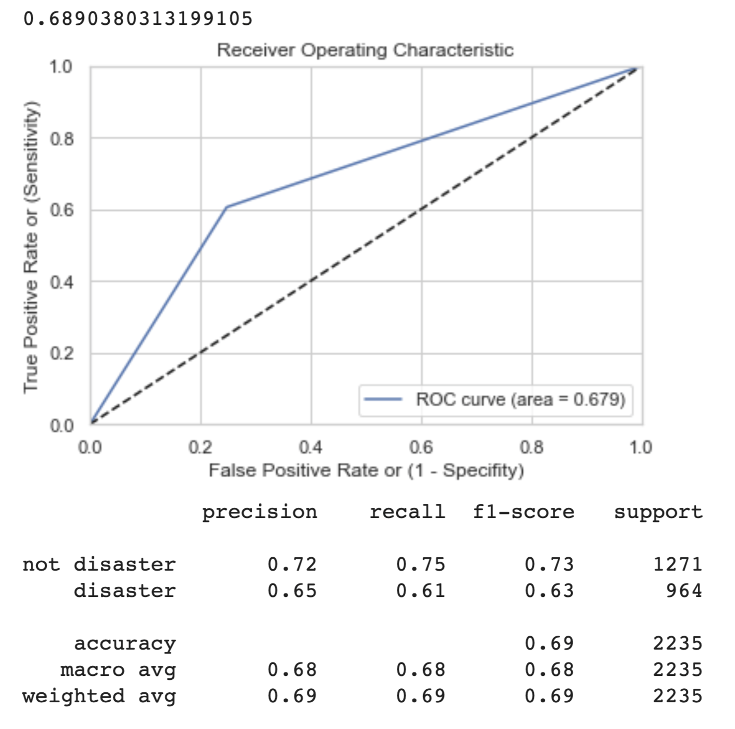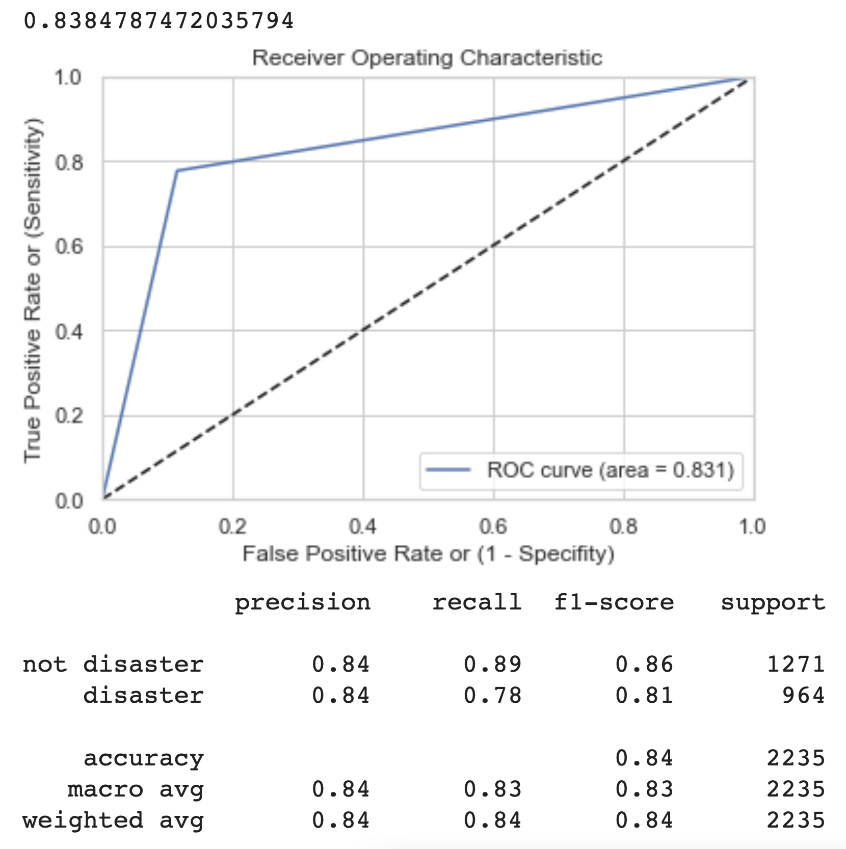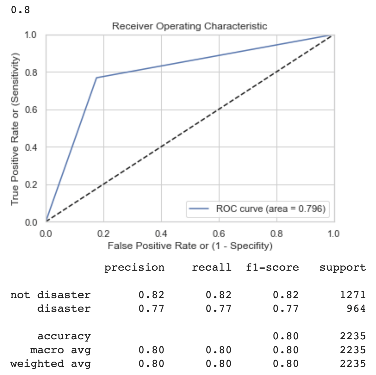We can see from the graphs and output above that the light BERT model performs the best in a variety of metrics. The ROC curve is the most towards the top left, indicating a low false positive rate and high true positive rate. This is a reflection of the higher precision and recall scores, meaning the model is more often, of those it predicts positive, getting true positives, and of those which are positive, it is getting most of the predictions largely correct (precision and recall, respectively).

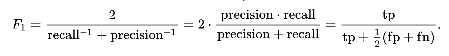
The f1-score is the harmonic mean of the precision and recall. It is a good way to calibrate how well we are classifying overall. However, it balances precision and recall equally in its formula. In the case in which we are actually detecting disasters occurring, we are more afraid of false negatives (type II error) because we would rather flag more disasters than less, especially when human lives are at stake.

The overall test set accuracy of the Light Data Cleaning BERT Model is 84%, which is a strong indicator of how it will perform on the unseen Kaggle competition test dataset.

Kaggle Submission

To test the model on the Kaggle Competition dataset, we predict the labels of the cleaned test data that we aren’t provided the labels of.

# actual test predictions
real_pred = bert_model.predict(test_tokenised_text_df)
# this is output as a tensor of logits, so we use a softmax function
real_tensor_predictions = tf.math.softmax(real_pred.logits, axis=1)
# this outputs the related probabilities of being disaster vs. non-disaster

# so we then use an argmax function to label
real_predictions = [list(bert_model.config.id2label.keys())[i] for i in tf.math.argmax(real_tensor_predictions, axis=1).numpy()]

Finally, we can submit the predictions! Locating the submission file downloaded from Kaggle, we can overwrite it with our own predictions:

# use utils function to get submission file in folder
utils.kaggle_submit(real_predictions, 'submission-light.csv')

To submit, we use the Kaggle API and type the following:

kaggle competitions submit -c nlp-getting-started -f submission-light.csv -m "YOUR OWN MESSAGE"

Conclusion

From Part 1 and Part 2, we have gone through a process of cleaning text data, extracting features from it, using typical pre-processing methods, and finally tested different machine learning methods for classifying disaster from non-disaster. The result demonstrates the power of pre-trained BERT models in using contextual information contained within text data. Specifically, we found out that heavy cleaning of text data actually works worse when input into a BERT model, because this contextual information is lost. Most importantly, by following the steps taken in this article, anyone can take their first steps towards understanding what it takes to achieve competitive results in a Kaggle competition. To improve accuracy further, one should attempt to tune the pre-trained BERT model further, perhaps use Large BERT, and could consider implementing the meta-feature data as an additional layer in the model to provide another dimension of training data.

If you liked this article follow me on Twitter! I am building every day.

Thanks for reading!

Bibliography

Kaggle Team, Natural Language Processing with Disaster Tweets, (2021), Kaggle Competitions

G. Evitan, NLP with Disaster Tweets: EDA, cleaning and BERT, (2019), Kaggle Notebooks

S. Theiler, Basics of using pre-trained GloVe Vectors, (2019), Analytics Vidhya

IA. Khalid, Cleaning text data with Python, (2020), Towards Data Science

A. Pai, What is tokenization?, (2020), Analytics Vidhya

G. Giacaglia, How Transformers Work, (2019), Towards Data Science

J. Devlin and M-W. Chang, Google AI Blog: Open Sourcing BERT, (2018), Google Blog

P. Prakash, An Explanatory Guide to BERT Tokenizer, (2021), Analytics Vidhya

J. Zhu, SQuAD Model Comparison, (n.d.), Stanford University

Alexander Bricken

Travelling the world.

Tweet Share Share