Does BERT Need Clean Data? Part 1 – Data Cleaning.

Detecting disasters 84% of the time and testing NLP methods.

If I describe Beyoncé’s Met Gala dress as a “hurricane”, does Hurricané Beyonce become a thing?

Introduction

In this article, we use the Disaster Tweets Competition dataset on Kaggle to learn typical data science & machine learning practices, and more specifically about Natural Language Processing (NLP). By applying different methods of text cleaning and then running Bidirectional Encoder Representations from Transformers (BERT) to predict disasters from regular Tweets, we can compare models and see how much text cleaning affects accuracy. The end result is a top 50 submission in the competition at ~84%.

What I hope you’ll learn about by reading this post includes the following:

• Exploring typical data science and machine learning practices by doing the following: importing, exploring, cleaning, and preparing data for machine learning.
• Applying specific NLP data preparation techniques such as feature engineering by creating meta-features and text cleaning using tokenisation.
• Applying BERT, a state-of-the-art language model for NLP, and figuring out what the best input for a BERT model is.

Objective

The main objective of this project is to distinguish Tweets that indicate a world disaster, from those that include disaster words but are about other things outside of disasters. By doing so, we can understand the way input text affects BERT; specifically if the text being more or less cleaned makes a difference!

It’s a difficult problem to solve because a lot of “disaster words” can often be used to describe daily life. For example, someone might describe shoes as “fire” which could confuse our model and result in us not picking up on actual fires that are happening around the world!

So, without further ado, let’s dive into our method for tackling this exciting problem!

Method

To summarise, the project is broken down into four notebooks. The first one contains essential data preparation, and the the subsequent notebooks (2, 3, & 4) are all different methods for obtaining our predictions.

Notebook 1 (Data Preparation):

1. Importing Libraries
2. Importing Data
3. Data Exploration
4. Data Preparation
5. Calculating Meta-Features

Notebook 2 (Meta-Feature DNN):

1. Import Prepared Data
2. Normalisation
3. Deep Neural Network
4. Model Evaluation & Submission

Notebook 3 (Heavy Cleaning BERT):

1. Import Prepared Data
2. Heavy Clean Text With Regular Expressions
3. Lemmatization
4. Tokenization
5. BERT Modelling
6. Model Evaluation & Submission

Notebook 4 (Light Cleaning BERT):

1. Import Prepared Data
2. Light Clean Text With Regular Expressions
3. Tokenization
4. BERT Modelling
5. Model Evaluation & Submission

Note: to see the full code for this project, see the GitHub repository here.

Data Preparation

Importing Data

To import our data, we write the following after downloading it and placing it in the correct directory:

raw_test_data = pd.read_csv("../data/raw/test.csv")
raw_train_data = pd.read_csv("../data/raw/train.csv")

# check your output by just running the following:
raw_train_data

Data Exploration

To explore our data, we use Pandas Profiling. This is a useful library for quickly getting a lot of descriptive statistics for the data we just imported.

profile = ProfileReport(raw_train_data, title="Pandas Profiling Report")
profile.to_notebook_iframe()

This should load up a nice widget to explore within your Jupyter Notebook. It will provide you with some great descriptive statistics, such as this!

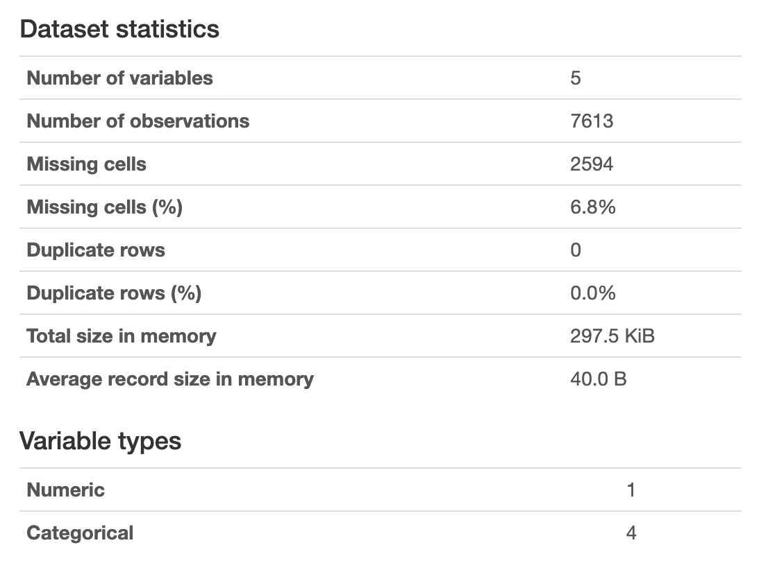
Specifically, by using Pandas Profiling we can check through some essential features of the dataset:

• Class distribution of target variable in the train dataset. This is a 4342 (0), 3271 (1) split. This near equal separation is ok for training our model.
• Missing data. We see that the location and keyword columns contain missing data. This will be handled below.
• Cardinality. Our location values are particularly distinct. This is also discussed and handled below.

From here, we can move on to our data preparation and deal with these problems we have highlighted!

Data Preparation

location and keyword contain null values, as demonstrated by the pandas profiling report.

We handle this by first examining the number of null values deeper.

foo = [(raw_train_data[['keyword', 'location']].isnull().sum().values, raw_test_data[['keyword', 'location']].isnull().sum().values)]

out = np.concatenate(foo).ravel()

null_counts = pd.DataFrame({
"column": ['keyword', 'location', 'keyword', 'location'],
"label": ['train', 'train', 'test', 'test'],
"count": out
})

sns.catplot(x="column", y="count", data=null_counts, hue="label", kind="bar", height=8.27, aspect=11.7/8.27)
plt.title('Number of Null Values')
plt.show()

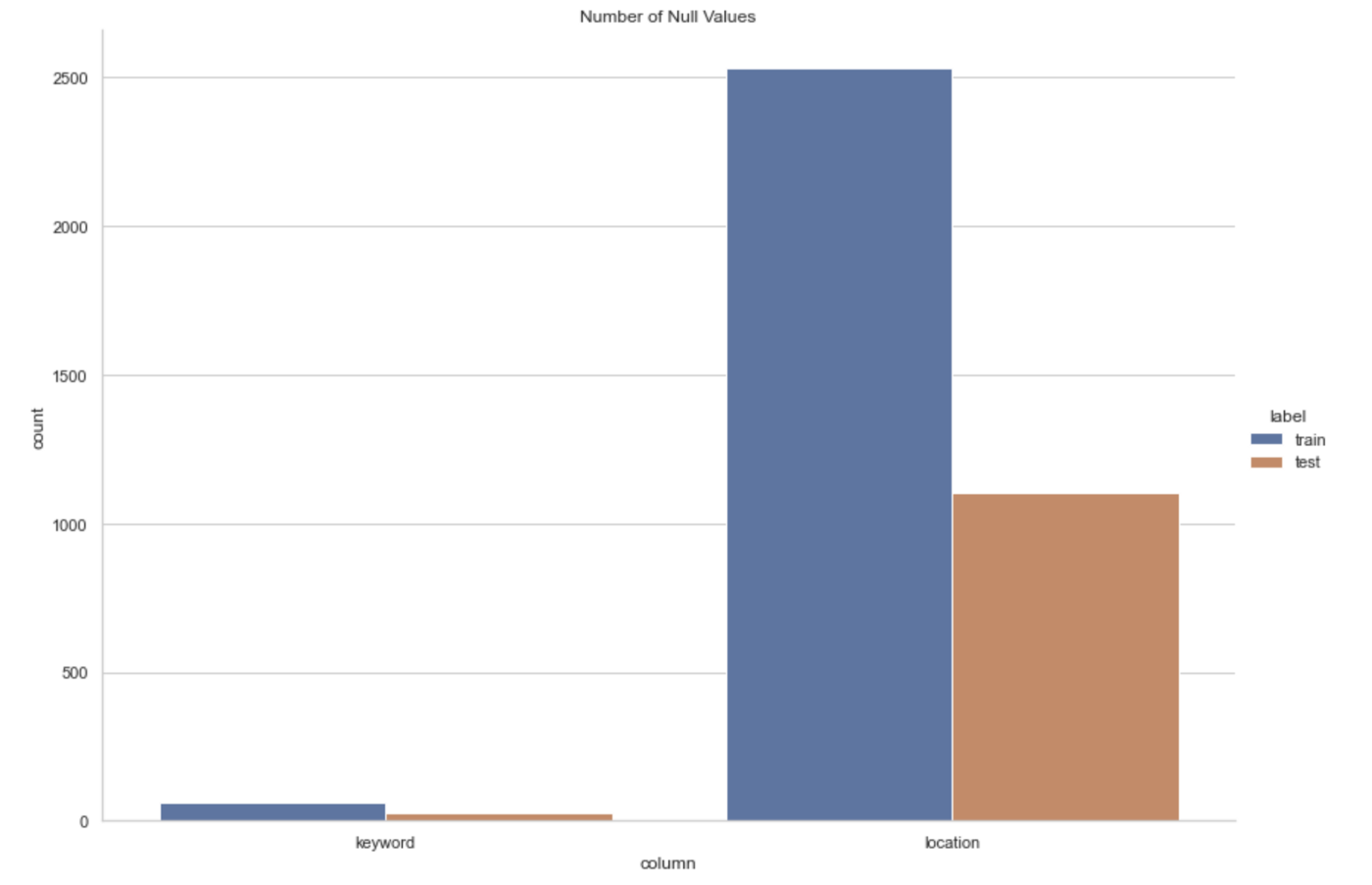
Locations from Twitter are user-populated and are thus too arbitrary. There are too many unique values and no standardization of input. We can remove this feature.

# drop location data
clean_train_data = raw_train_data.drop(columns="location")
clean_test_data = raw_test_data.drop(columns="location")

Keywords, on the other hand, are interesting to consider as a way of identifying disasters. This is because some keywords really are only used in a certain context.

What do our keywords look like? We can output word clouds for our train and test datasets to examine this.

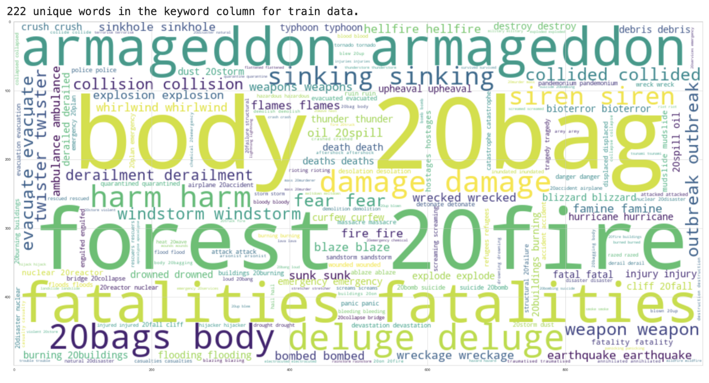
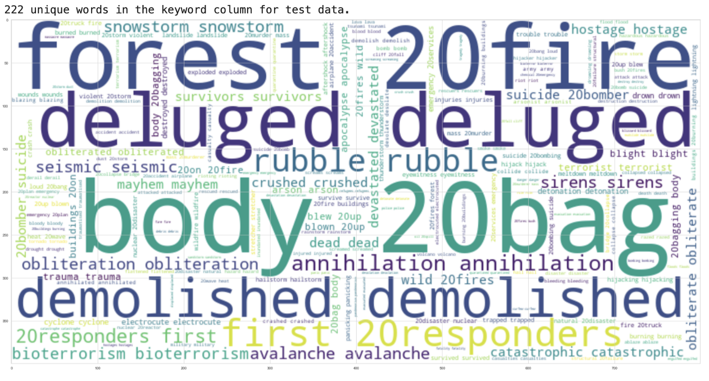
We see that there is a good level of overlap between the keywords in treatment and control. Keyword is just one way of looking at the data, and if we just examine keywords there is not enough context to generate accurate predictions. Likewise, because we are implementing a BERT model which is all about the context of a word in a sentence, we don’t want to do anything like add the keyword to the end of the associated Tweet to increase the weight of that word.

One clever way to leverage the keyword in our model is to convert the keyword into a sentiment score. This way, we have a value that acts as a meta-feature, without altering the important information contained in the Tweets. We do this by using NLTK library’s built-in, pretrained sentiment analyzer called VADER (Valence Aware Dictionary and sEntiment Reasoner).

# drop nan keyword rows in train dataset
clean_train_data = clean_train_data.dropna(subset=['keyword']).reset_index(drop=True)

# we fill none into the Nan Values of the test dataset, to give 0 sentiment
clean_test_data['keyword'] = clean_test_data['keyword'].fillna("None")

# collect keywords into arrays
train_keywords = clean_train_data['keyword']
test_keywords = clean_test_data['keyword']

# use sentiment analyser
sia = SentimentIntensityAnalyzer()
train_keyword_sia = [sia.polarity_scores(i)['compound'] for i in train_keywords]
test_keyword_sia = [sia.polarity_scores(i)['compound'] for i in test_keywords]

# update keyword column
clean_train_data['keyword'] = train_keyword_sia
clean_test_data['keyword'] = test_keyword_sia

Finally, we check for duplicate data and the corresponding labels of the duplicates.

# check for duplicates using groupby
df_nondupes = clean_train_data.groupby(['text']).nunique().sort_values(by='target', ascending=False)

# find duplicates with target > 1 as a way of flagging if they are duplicate
df_dupes = df_nondupes[df_nondupes['target'] > 1]
df_dupes.rename(columns={'id':'# of duplicates', 'target':'sum of target var'})

We see there are some duplicates. We don’t want any duplicates when training our model because it can bias our output. These would be particularly bad if they are labelled differently as well. From the output, we can see they are. This is extra confusing for the model to have something with the same features but a different label.

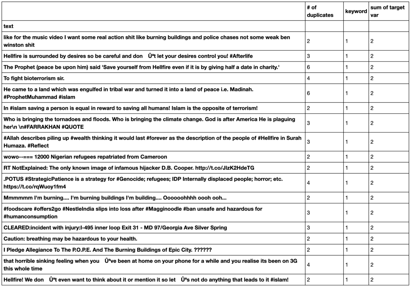
If we iterate through these duplicates we can individually label them by hand so we keep the data. This is necessary because some of them are mislabeled as well as being duplicate. For example, there are three duplicates of the first row, but 2 of them have the target label 1, and one of them has target label 0. This is seen throughout the table via the difference in the the # of duplicates against the sum of target var, as seen above.

# take index which is the texts themselves 
dupe_text_list = df_dupes.index dupe_text_list = list(dupe_text_list) 
# turn into list

# manually make label list to iterate 
right_labels = [0,0,0,1,0,0,1,0,1,1,1,0,1,1,1,0,0,0]

# drop duplicates except for one
clean_train_data = clean_train_data.drop_duplicates(subset=['text'], keep='last').reset_index(drop=True)

# relabel duplicate rows
for i in range(len(dupe_text_list)):
    clean_train_data.loc[clean_train_data['text'] == dupe_text_list[i], 'target'] = right_labels[i]

Calculating Meta-Features

Now that our data is cleaned and prepared, we are on to the fun stuff!

We need ways to learn more about our data and separate it out into additional features. By thinking about different variables we can generate that might help us distinguish disasters from non-disasters, we can train our model on more features. This will provide more visibility for our model. The best way to think about Tweets indicating disaster is that they are likely from higher quality sources that are more serious in nature. Thus, following stricter grammatical rules, fully reporting on the situation, and sharing links. The following meta-features, alongside our sentiment score calculated from the keywords column, will be proxies for the types of Tweets we are looking for (cherry-picked from here).

• num_hashtags - count of hashtags (#) (hypothesis (H): hashtags are used by normal users rather than new agencies)
• num_mentions - count of mentions (@) (H: more tags could be used by normal users rather than news agencies)
• num_words - count of words (H: more words in proper reports on Twitter than normal user tweets)
• num_stop_words - number of stop words (H: more stop words used via proper grammar from news agencies)
• num_urls - count of urls (H: urls shared by news agencies reporting disaster more often than not)
• avg_word_length - average character count in words (H: longer words that aren’t abbreviated used by news agencies)
• num_chars - count of characters (H: more characters used in news agency tweets to report full story)
• num_punctuation - count of punctuations (H: more punctuation in news agency tweets following correct grammar)

We use this code to construct these features.

### num_hashtags
clean_train_data['num_hashtags'] = clean_train_data['text'].apply(lambda x: len([c for c in str(x) if c == '#']))
clean_test_data['num_hashtags'] = clean_test_data['text'].apply(lambda x: len([c for c in str(x) if c == '#']))

### num_mentions
clean_train_data['num_mentions'] = clean_train_data['text'].apply(lambda x: len([c for c in str(x) if c == '@']))
clean_test_data['num_mentions'] = clean_test_data['text'].apply(lambda x: len([c for c in str(x) if c == '@']))

### num_words
clean_train_data['num_words'] = clean_train_data['text'].apply(lambda x: len(str(x).split()))
clean_test_data['num_words'] = clean_test_data['text'].apply(lambda x: len(str(x).split()))

### num_stop_words
clean_train_data['num_stop_words'] = clean_train_data['text'].apply(lambda x: len([w for w in str(x).lower().split() if w in STOPWORDS]))
clean_test_data['num_stop_words'] = clean_test_data['text'].apply(lambda x: len([w for w in str(x).lower().split() if w in STOPWORDS]))

### num_urls
clean_train_data['num_urls'] = clean_train_data['text'].apply(lambda x: len([w for w in str(x).lower().split() if 'http' in w or 'https' in w]))
clean_test_data['num_urls'] = clean_test_data['text'].apply(lambda x: len([w for w in str(x).lower().split() if 'http' in w or 'https' in w]))

### avg_word_length
clean_train_data['avg_word_length'] = clean_train_data['text'].apply(lambda x: np.mean([len(w) for w in str(x).split()]))
clean_test_data['avg_word_length'] = clean_test_data['text'].apply(lambda x: np.mean([len(w) for w in str(x).split()]))

### num_chars
clean_train_data['num_chars'] = clean_train_data['text'].apply(lambda x: len(str(x)))
clean_test_data['num_chars'] = clean_test_data['text'].apply(lambda x: len(str(x)))

### num_punctuation
clean_train_data['num_punctuation'] = clean_train_data['text'].apply(lambda x: len([c for c in str(x) if c in string.punctuation]))
clean_test_data['num_punctuation'] = clean_test_data['text'].apply(lambda x: len([c for c in str(x) if c in string.punctuation]))

Remember, you can write clean_train_data and run the cell to see what our current pandas dataframe looks like!

At this point, we have cleaned up the null variables from the dataset, calculated our meta-features, and gotten rid of mislabels and duplicates.

We should save our datasets. We do this by using pickles!

# we save these as pickles
clean_train_data.to_pickle("../data/pickles/clean_train_data.pkl")
clean_test_data.to_pickle("../data/pickles/clean_test_data.pkl")

We can now do the following:

• Lightly clean the text data, without removing stopwords or other contextual pieces of the Tweets, and then run BERT.
• Heavily clean the text data, removing stopwords and other features that might confused the model, and then run BERT.
• Separate the meta-features from the text data and try running a Deep Neural Network.

From there, we can compare the accuracy of our models appropriately. Because BERT is a language model that utilises the structure of the sentence from both directions to connect every output element to every input element, and dynamically adjust weightings depending on this connection (this process is called attention), my hypothesis is that the lighter pre-processing will do better. This is because stopwords and other grammatical features of sentences may have a part to play in helping the model’s attention. In other words, BERT avoids assigning words fixed meanings independent of context. Rather, words are defined by their surroundings words.

Next Steps

Where we generate predictions and learn more about BERT, machine learning, and how our data cleaning process affects outcomes, see Part 2 here or on Medium.

If you liked this article follow me on Twitter! I am building every day.

Thanks for reading!

Bibliography

Kaggle Team, Natural Language Processing with Disaster Tweets, (2021), Kaggle Competitions

G. Evitan, NLP with Disaster Tweets: EDA, cleaning and BERT, (2019), Kaggle Notebooks

S. Theiler, Basics of using pre-trained GloVe Vectors, (2019), Analytics Vidhya

IA. Khalid, Cleaning text data with Python, (2020), Towards Data Science

A. Pai, What is tokenization?, (2020), Analytics Vidhya

G. Giacaglia, How Transformers Work, (2019), Towards Data Science

J. Devlin and M-W. Chang, Google AI Blog: Open Sourcing BERT, (2018), Google Blog

P. Prakash, An Explanatory Guide to BERT Tokenizer, (2021), Analytics Vidhya

J. Zhu, SQuAD Model Comparison, (n.d.), Stanford University

Alexander Bricken

Travelling the world.

Tweet Share Share